Cross-modal Scene Graph Matching for Relationship-aware Image-Text Retrieval

Overview

Natural scenes image mainly involves two kinds of visual concepts: object and their relations, which are equally essential to image-text retrieval. Intuitively, compared to CNN-based methods, Graph-based image feature contains more important visual information and considers the relationship between objects.

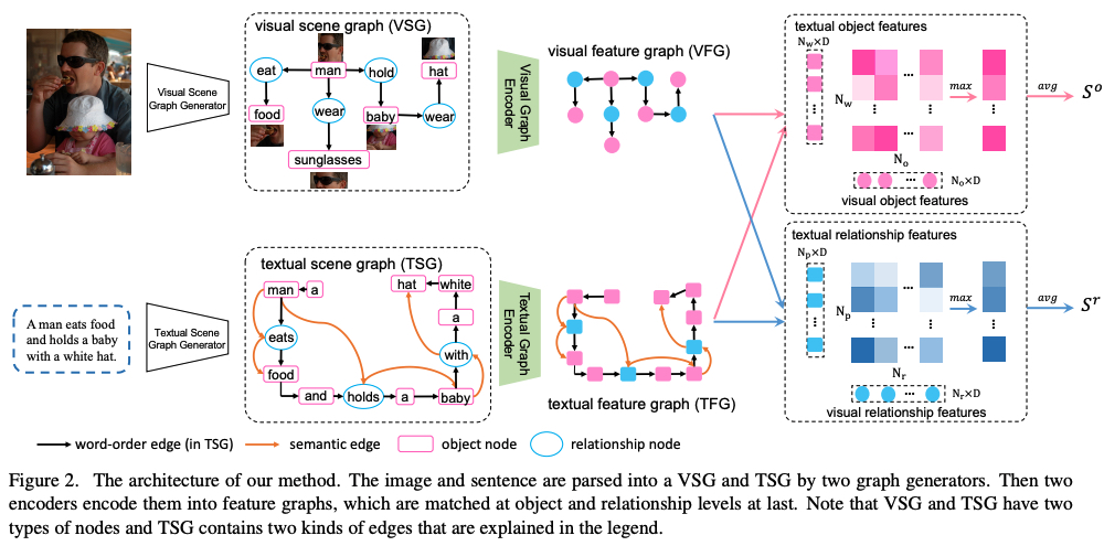
This paper use represent image and text with respectively visual scene graph (VSG) and textual scene graph (TSG), then CMIR tasks is naturally formulated as cross-modal scene graph matching.

This method enables us to obtain both object-level and relationship-level cross-modal features, which favorably enables us to evaluate the similarity of image and text in the two levels in a more plausible way.

Motivation and Contributions

alt img

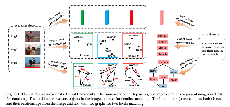
As shown in the top of the figure, early approaches use global representations to express the whole image and sentence, which ignore the local details. These methods work well on simple cross-modal retrieval scenario, but not performance good at more realistic cases that involve complex natural scenes.

Recent studies pay attention to local detailed matching by detecting objects in both images and text, but ignore the relationships.

In this paper, authors organize the objects and the relationships into scene graphs for both modalities, converting the conventional image-text retrieval problem to the matching of two scene graphs.

Contributions

Extract objects and relationships from the image and text to form the VSG and TSG, and design a so-called Scene Graph Matching (SGM) model.
The VSG encoder is a Multi-modal Graph Convolution Network (MGCN), which enhances the representations of each node on the VSG by aggregating useful information from other nodes and updates the object and relationship features in different manners.
The TSG encoder contains two different bi-GRUs aiming to encode the object and relationship features, respectively.
Both object-level and relationship-level features are learned in each graph, and the two feature graphs corresponding to two modalities can be finally matched at two levels in a more plausible way.

Methodology

Visual Scene Graph Generation

alt img

Given a raw image, represent a visual scene graph as $G = \{V, E\}$, $V$ is the node-set, and $E$ is the edge-set. As shown in figure, the pink rectangles denote object nodes, each of which corresponds to a region of the image. The ellipses in light blue are relationship nodes, each of which connects two object nodes by directed edges.

If there are $N_o$ object nodes and $N_r$ relationship nodes in VSG:

Object nodes set:

\[O = \{o_{i}|i = 1,2,...,N_o \}\]

Relationship nodes set: $R = \{r_{ij}\} \subseteq O \times O$, $\vert R \vert = N_r$, $r_{ij}$ is the relationship of $o_i$ and $o_j$

Visual Scene Graph Encoder

alt img

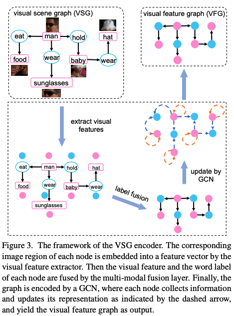
Visual Feature Extractor. The pre-trained visual feature extractor: emcoding image regions into feature vector (Faster-RCNN). Each node in VSG will be encoded into a $d_1$-dimension visual feature.

For object node $o_i$, visual feature vector $v_{oi}$ is extracted from its corresponding image region.

For relationship node $r_{ij}$ , visual feature vector $r_{ij}$ is extracted from the union image region of $o_i$ and $o_j$ .

Label Embedding Layer.

Given one-hot vectors $l_{oi}$ and $l_{r_{ij}}$, output $e_{oi}$ and $e_{r_{ij}}$ :

$W_o \in R^{d_2 \times C_o}$ and $W_r \in R^{d_2 \times C_r}$ are trainable parameters and initialized by word2vec ($d_2=300$). $C_o$ is the category number of objects and $C_r$ is the category number of relationships.

\[e_{oi} = W_oI_{oi} , W_o \in R^{d_2 \times C_o}\] \[e_{r_{ij}} = WrI_{r_{ij}}, W_r \in R^{d_2 \times C_r}\]

Multi-modal Fusion Layer.

$W_u \in R^{d_1 \times (d_1 + d_2)}$ is the trainable parameter of fusion layer.

$u_{oi} = tanh(W_u[v_{oi},e_{oi}])$,

\[u_{r_{ij}} = tanh(W_u[v_{r_{ij}},e_{r_{ij}}])\]

Visual Scene Graph Encoder

alt img

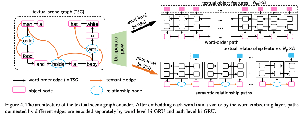
Two relationshps: word order (black arrows) and semantic relationship (brown arrows, are built from SPICE)

The textual scene graph encoder consists of a word embedding layer, a word-level bi-GRU encoder, and a path-level biGRU encoder.

Build TSG:

Fiest, each word $w_i$ in the sentences is embedded into a vector by the word embedding layer as $e_{w_{i}} = W_el_{w_{i}}$ . ($l_{w_{i}}$ is the one-hot vector of $w_i$ , $W_e$ is the parameter matrix of embedding layer, initialisation as the same word2vec in VSG encoder and be learned during training end-to-end).

Second, two kinds of path are encoded separately by different bi-GRUs.

For the word-order path:

\[\overrightarrow{h_{w_{i}}} = \overrightarrow{GRU_w}(e_{w_{i}},\overrightarrow{h_{w_{i-1}}})\] \[\overleftarrow{h_{w_{i}}} = \overleftarrow{GRU_w}(e_{w_{i}},\overleftarrow{h_{w_{i+1}}})\] \[h_{w_{i}} = (\overrightarrow{h_{w_{i}}} + \overleftarrow{h_{w_{i}}})/2\]

For the $N_p$ semantic relationship paths:

$h_{p{i}} = (\overrightarrow{GRU_p}(path_i) + \overleftarrow{GRU_p}(path_i))/2, i \in [1,N_p]$ , the last hidden state feature of $i-th$ semantic relationship path, which is also a relationship feature of the TSG.

Similarity Function

Each graph has two levels of features, this work match them respectively.

Setting:

there are $N_o$ and $N_w$ object features in the visual and textual feature graph, each of them is a $D$-dimension vector.
for feature vectors $h_i$ and $h_j$ , the similarity score is $h_{i}^{T}h_{j}$, the similarity scores of V and T objects, it’s a $N_w \times N_o$ matrix.
find the maximum value of each row, which means for very textual object, the most related visual objects among $N_o$ visual objects is picked up.
similarity score:
- \[S^{o} = (\sum_{t=1}^{N_w} \max_{i \in [1, N_o]} h_{w_t}^{T}h_{o_i})/N_{w}\]
- \[S^{r} = (\sum_{t=1}^{N_p} \max_{r_{ij} \in R} h_{p_t}^{T}h_{r_{ij}})/N_{p}\]
- \[S = S^o + S^r\]

Loss Function

usually, use triplet loss:

\[L(k,l) = \sum_{\hat{l}} max(0,m- S_{k \hat{l}} + S_{k\hat{l}}) + \sum_{\hat{k}} max(0,m- S_{k \hat{l}} + S_{k\hat{l}})\]

Consider to the influence of hardest negative samples,

\[L_{+}(k,l) = max(0, m - S_{kl} + S_{k \hat{l}}) + max(0, m - S_{kl} + S_{\hat{k} l})\]

where $\hat{l} = argmax_{j \not = l}S_{kj}$ and $k' = argmax_{j \not = k}S_{jl}$ are hardest negative in the mini-batch.